|
Simatest: Overview – Introduction to Simatest — recommended for getting started Simatest ISP/Camera Simulator — Instructions and Reference Image Sensor Noise – measurement and modeling – using raw files for image sensor Dynamic Range and Simatest Using Color/Tone Interactive – Interactive analysis of color & grayscale test charts Color/Tone & eSFR ISO noise measurements – describes how to measure image sensor noise from raw images Dynamic Range – a general introduction with links to Imatest modules that calculate it Image information metrics – new measurements, based on Shannon information theory, that are superior predictors of Machine Vision system performance. |
Introduction – Simatest block diagram – Modeling image sensor noise – Measuring the noise
Simulating the noise – Low light performance – Modeling and measuring image sharpness
Simulating image sharpness – Simulating camera JPEGs – Summary
This page contains several examples showing how to use Simatest — Imatest’s camera and Image signal processing simulator — for modeling and measuring camera system performance. This post is intended to supplement Simatest — ISP/Camera Simulator — Overview, which we recommend reading first.
Simatest is available as part of Imatest 25.1
Introduction
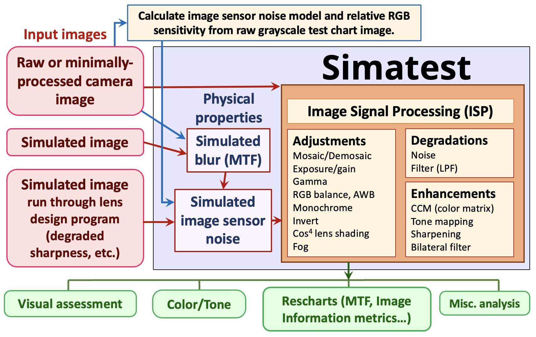
Simatest can model and measure the effects of Image Signal Processing (ISP) starting with
- Raw or minimally-processed camera images (demosaiced or not) — which can also be analyzed by Color/Tone to measure image sensor noise or SFR to measure lens blur (which can be simulated in Simatest with a gaussian blur).
- Simulated (test chart) images, which should be blurred to match the MTF (SFR) of raw camera images, typically using a simple gaussian or Airy disk filter. Must also include image sensor noise, which is introduced in the Overview and described in detail on this page.
- Simulated images degraded by a lens design program. This enables the “soft prototyping” of a camera before the hardware is specified and built. Image sensor noise must be added.
Test chart images are used where quantitative results (MTF, information metrics, SNR, etc.) are needed, but any image can be used. An ISP pipeline can be applied to images from any source.
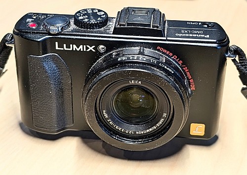 Two cameras were used for examples on this page:
- the Panasonic Lumix LX5, an older (2010) 10.1 megapixel compact digital camera with 2.14 μm pixel pitch and a high quality Leica-branded zoom lens. Its image processing is simple by 2025 standards — it has no Computational Imaging or Artificial Intelligence, and most importantly, it has (undemosaiced) raw output.
- The Sony A6000, a 24 MP Micro Four-Thirds camera with a 3.88 μm pixel pitch and an excellent Canon 60mm macro lens, which we use for measuring test chart quality.
We will show how to
- Model the image sensor noise using a raw image of a grayscale test chart.
- Calculate how camera performance varies with Exposure Index (EI; widely known as ISO speed), where increasing the EI is equivalent to decreasing the sensor illumination.
- Model the approximate camera spatial domain response, including MTF (SFR).
Modeling image sensor noise
|
The full description of Image sensor noise is in Image Sensor Noise – measurement and modeling. It is also referenced in Simatest — Overview. |
A key step — perhaps the most important step — in simulating digital camera performance is to model and measure the image sensor noise, which consists of dark noise from several sources, photon (or electron) shot noise, and PRNU (photo response nonuniformity). The Simatest model is derived from measurements of raw images of grayscale test charts, preferably transmissive charts, which have much larger tonal ranges than reflective charts.
Once an image sensor’s noise has been properly characterized, Simatest can be used to predict camera performance for a wide variety of camera configurations — lenses, illumination, image processing, etc.
For linear (non-HDR) image sensors, noise can be derived from the Digital number (pixel level DN ) of the signal + noise at the image sensor.
DN = DNmeas – DNoff where DNoff is an offset frequently included in undemosaiced image files.
Estimating DNoff , which is common in undemosaiced raw files, is described below and in Black level offset and saturation level. It is normally not present in demosaiced files, and it can be effectively removed from raw images by checking Optimize in the More settings window.
The equation for image sensor noise, σN, uses the normalized Digital Number, V = DN / DNmax, as described in Image sensor noise model — equations.
\(\sigma_N = \sqrt{k_{Ndark}^2 + k_{Nshot}^2 V + k_{FPN}^2 V^2}\)
This model is based on the noise models in the EMVA 1288 standard for linear sensors, section 2.4 and James R. Janesick, “Photon Transfer DN → λ”, SPIE Press, 2007, chapter 5.
Measuring the image sensor Noise
kNdark , kNshot , and kFPN are the key parameters for the Simatest image sensor noise model. Measurements must be made carefully from raw (undemosaiced and unprocessed) images.
The steps for measuring the noise
- Acquire an image of a grayscale test chart, preferably a transmissive chart designed for measuring dynamic range.
- Save the image in an undemosaiced raw format.
- Read the raw image into Color/Tone Interactive without demosaicing. (Color Tone Auto also works, but is less flexible.)
- For commercial raw files, the LibRaw settings window will open. The Bayer RAW 16-bit linear preset is recommended. The converted image is saved as a TIFF. Details in Image Sensor Noise.
- For binary files (mostly from development systems), use Generalized Read Raw, which needs to be set up to recognize the file extension and associate it with the input and output pixel size, the image width and heights, and several optional parameters. Demosaicing should be set to None. Details in Image Sensor Noise.
- Since the undemosaiced image is monochrome, the Standard monochrome or Bayer RAW? box will appear. Select the appropriate Pixel color mapping (Red in R1C2 (GR/BG) for the Lumix LX5; R1C1 for the A6000). (If the image contains recognizable color, you can open it in Rawview to determine the color mapping.) Then select (Analyze image as) Bayer RAW (undemosaiced). This table has mappings for several cameras in our lab. Canon and Sony cameras are usually R1C1 (RGGB), but Panasonic Lumix cameras are all over the place.
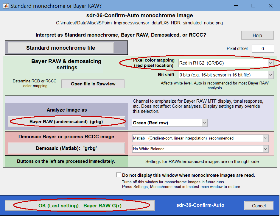 Standard Monochrome or Bayer Raw? settings window
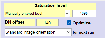 Estimate the Black Level offset, DNoff and saturation level using techniques described in Black level offset and saturation level. DNoff can be larger than the smallest DN (image pixel level) but must be smaller than the DN of the darkest patch; it’s OK for the starting guess to be 0.
Check the Optimize checkbox to the right of DN Offset in the Color/Tone settings to obtain a refined value for DNoff . Photon Transfer Plots 10-12, which show noise and SNR as a function of pixel level, contain the key results, which are not sensitive to the exact value of DNoff . For the Lumix LX5, the EXIF data says offset is 128 and the saturation level is 4095, but the actual offset is closer to 142.- Press OK when your settings are complete. A Levenberg-Marquardt optimizer will be run to find the values of kNdark, kNshot, and kFPN (the coefficients for dark noise, photon shot noise, and fixed-pattern noise) that best match the data to enter into Simatest.
- Select Display 10. Noise analysis to display a plot of the noise as a function of Digital Number: the Photon Transfer Curve. The Dark, Shot, and Fixed Pattern (PRNU) noise coefficients are displayed in the text below the plot. SNR plots 11 or 12 are sensitive to DNoff + stray light, making them less useful than the simple noise plot.
![]() Photon Transfer Curve, similar to OnSemi Application Note AND9189/D
Photon Transfer Curve, similar to OnSemi Application Note AND9189/D
Measured and fit noise vs. normalized Digital Number for the LX5. Key results:
RGB Balance = 0.429 1.000 0.603; [Dark shot, …] = 0.0005498, 0.00985, 0.00615
The text below the plot contains two sets of results to enter into Simatest. The most important is [Dark, shot, FP noise coefficients for Simatest] = 0.0005498, 0.00985, 0.00615. The saturation (well) capacity of 7079 electrons (e-) corresponds to 38.5 dB SNR (a little lower than the measured SNR which includes the PRNU signal-dependent fixed-pattern noise). The DN offset (DNoff = 143) and saturation level (DNmax = 4095) must also be entered.
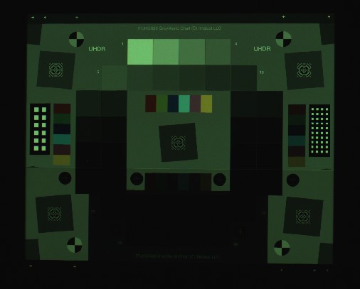 Another result of importance is RGB = 0.429 1.000 0.603, which represents the color of the middle gray patches, normalized to 1. Because of the light source and sensor sensitivity, the image (thumbnail shown on the left with no color correction) has a greenish tint.
More details of the noise calculations are in Image Sensor Noise – measurement and modeling and is also in Simatest — Overview.
Dark noise is actually a combination of several signal-independent noise sources, described in OnSemi Application Note AND9189/D. Electronic (Johnson) noise has a strong temperature dependence. It is proportional to (4kT)1/2. Dari current noise increases with exposure time.
We expect to extend the noise model to include multi-region HDR sensors by late 2025.
Simulating the image sensor noise
The measured parameters for photon shot noise noise, dark noise, and RGB balance can be entered into a Simatest model of the image.
- Open Simatest and read in an ideal test chart image file created by the Imatest Test Charts program. Our examples use two charts.
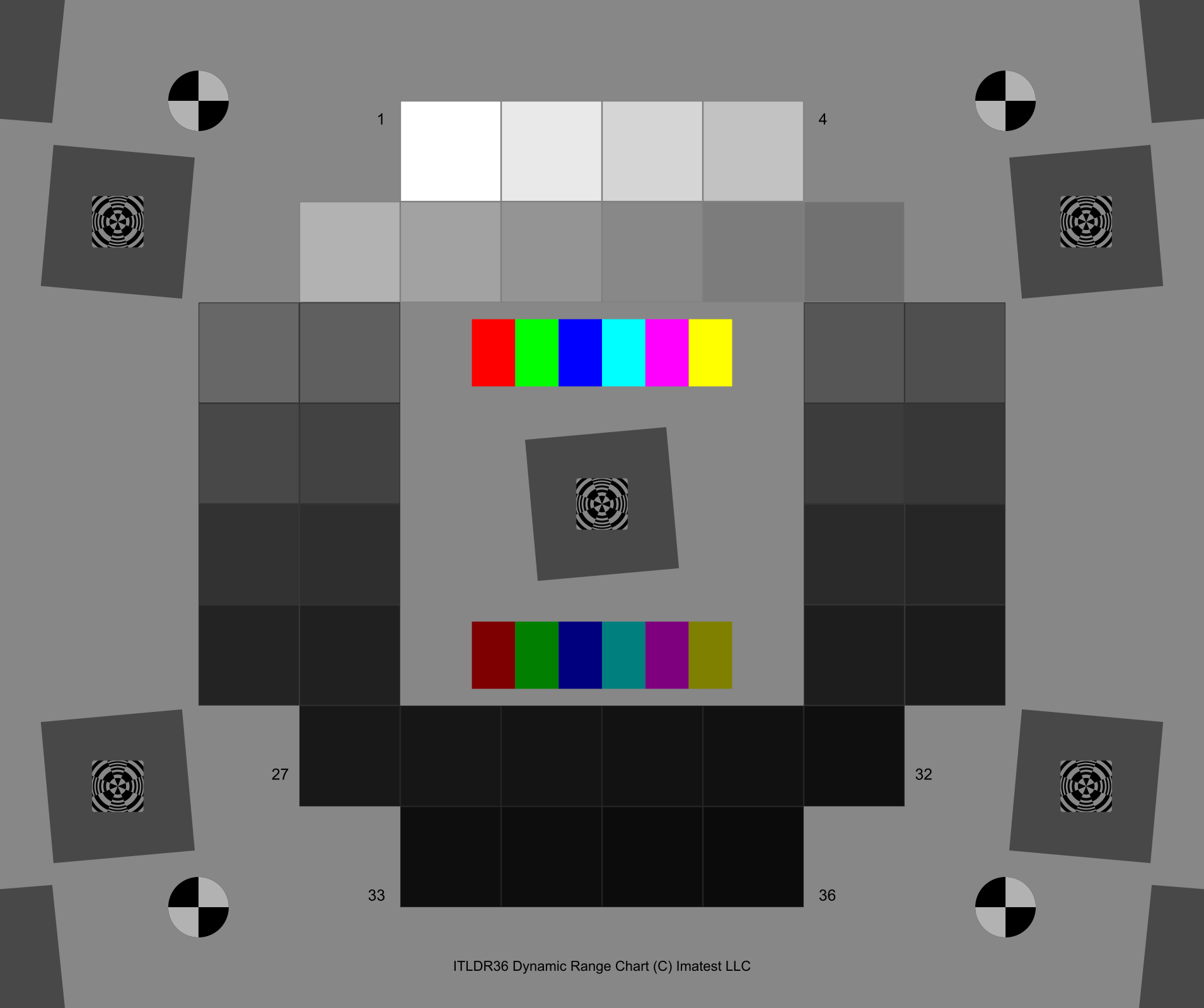
- an ideal 36-patch dynamic range test chart with density steps of 0.1 (maximum optical density = 3.5), available for download as a 16-bit depth PNG image here, and
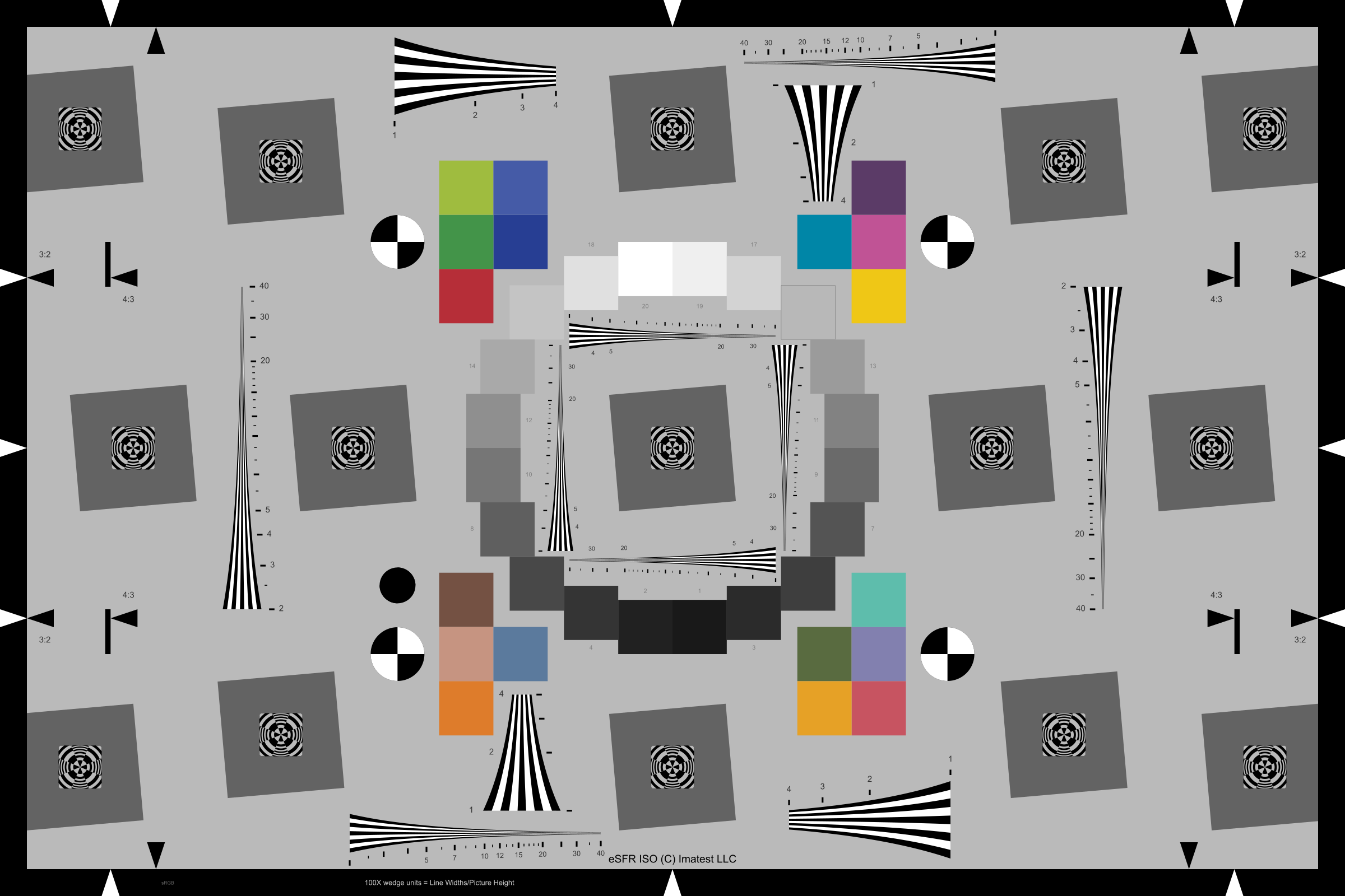
- an ideal 2400×1600 pixel Enhanced eSFR ISO 2017 chart, available for download as a PNG image here).
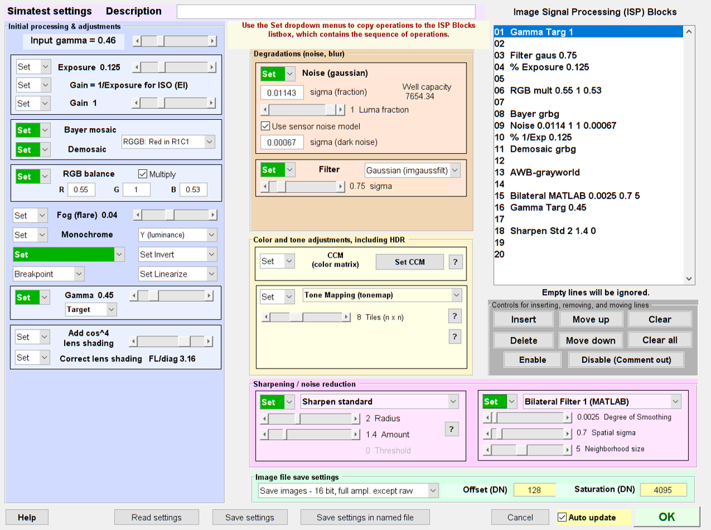
- Open the Simatest settings window, and enter the following settings to replicate the (undemosaiced) raw image we just measured.
[Input Gamma 0.45* ] A property of the input image. May depend on Test Charts settings, typically 0.45 or 1.
*Required for characterizing the input image. Not in the ISP Blocks list.
Gamma Targ 1 Linearizes the image, which has an initial gamma ≅ 1/2.2.
Filter gaus 0.75 Lowpass filters the image to approximate the lens blur.
RGB mult 0.43 1 0.60 Applies the measured color imbalance. Entered with the R, G, and B boxes in RGB Balance.
Bayer grbg Turns the RGB image into a synthetic Bayer raw image.
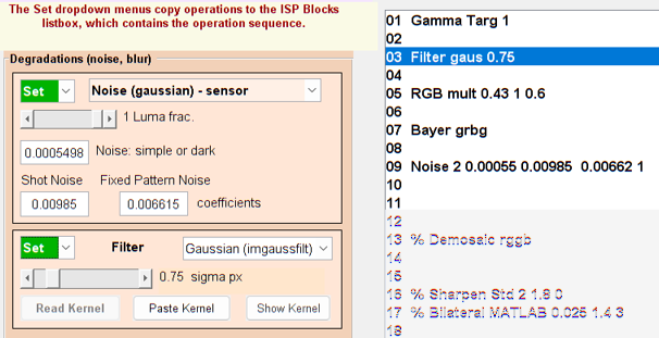
Noise settings consist of the following five entries.
Noise (Gaussian) – sensor (type 2)
Noise: dark: 0.0005498
Shot noise: 0.000985
Fixed pattern noise: 0.006615
Luma (noise) fraction: 1 (only for color images; unused for raw)
These five settings result in Noise 2 0.0055 0.00985 0.000662 1 in the ISP BLocks window, above-right.
These settings are listed in the large table in Simatest — instructions and reference. Settings prefixed by % are disabled (commented out).
Click OK when the settings are complete.
- Check Auto update in the lower-right of the Settings window, next to OK , to automatically update the calculations when OK is pressed. If Auto update is unchecked, you’ll need to press Update calculations in the main window. The resulting image will be a Bayer raw image.
- To get a raw image with the same offset and maximum value as the camera (142 and 4095 for the LX5), Set Save images – 16 bit depth, Offset (DN) 142, Saturation (DN) 4095 at the bottom-right of the settings window. (This only applies to raw images.)
- Open the image in Color/Tone Interactive, with the 36-patch Dynamic Range chart selected. Because the undemosaiced image file is monochrome, the Standard Monochrome or Bayer RAW? window will open. The key setting for the LX5 is Pixel color mapping = R1C2. Then press the Bayer RAW (undemosaiced) button.
- Select the ROIs or confirm the ROI selection, as required. The results will appear.
![]() Simulated noise vs. input pixel level the LX5 (2.14 μm pixels)
Simulated noise vs. input pixel level the LX5 (2.14 μm pixels)
The simulated noise is virtually identical to the measured noise (above), but the plots look different because the minimum x-axis value is 0.8×10⁻⁵ for the measured value vs. 2.6×10⁻⁴ for the simulation.
Low light performance
| This section illustrates how to calculate a camera’s key physical properties — image sensor noise coefficients, RGB balance, and approximate lens blur — and use them to predict the camera’s low light (high ISO speed) performance. |
Cameras use two strategies for low light conditions
- Increase the exposure time. This applies primarily to still cameras. Video cameras have limits on their maximum exposure times, typically around 1/30 second, depending on the application. For long exposures, dark current noise, which is measured in units of electrons per second of exposure (e-/s) in EMVA 1288, can be significant. As of April 2025, Imatest does not have a measurement of dark current noise, but it can use EMVA 1288 measurements by substituting iDark in e-/s and exposure time s into \(\displaystyle k_{NDark} = \sqrt{\sigma^2_{Dk}+DSNU^2 + (i_{Dark}\ s)^2} \times \text{Gain}(V/e-) \)
- Increase the analog gain, or equivalently, increase the ISO Speed (Exposure Index). Simatest simulates this by decreasing the signal, adding the image sensor noise, then restoring the signal to its original level.
Strategy for comparing low light measurements with simulations
The tests were performed on a Sony A6000 24 MP Micro Four-Thirds camera with 3.88 μm pixels set to ISO (EI) 100 (the minimum analog gain).
The steps below represent two parallel paths: Odd steps (1, 3, and 5) are measurements; even steps (2, 4, and 6) are the corresponding simulations. The key parameters describing the system, which are determined from the measurement, are
- the image sensor noise coefficients, measured in Color/Tone
- The RGB balance, measured in color/Tone
- The lens/sensor blur, determined iteratively by comparing the measured and simulated MTF curves in (Rescharts) SFR.
Once these parameters have been measured, camera performance can be simulated for a wide variety of conditions. This can save a lot of measurement time.
|
Step 1 – measurement. Photograph a grayscale test chart (preferably a transmissive dynamic range chart), save it in a raw format, then read it without demosaicing into Color/Tone for measuring the image sensor noise coefficients and RGB color balance.
|
|
Step 2 – simulation. Starting with
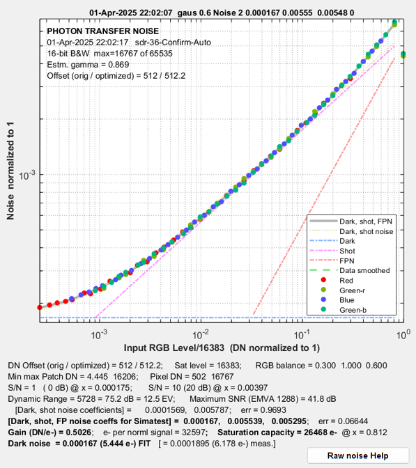
Run Simatest to simulate the image with noise, then open the simulated image with Color/Tone Interactive, which is very convenient from the Simatest window. The Photon Transfer Curves (PTCs), i.e., noise as a function of digital number, DN, are shown on the left and right, below. They are be very close, as expected. |
|
The key settings for calculated by Color/Tone for use in Simatest are noise coefficients, kNdark = 0.0001672, kNshot = 0.005554, kFPN = 0.005477; and RGB (balance) = 0.306, 1.0, 0.606. Simatest settings are shown on the right. The simulation results are on the right, below. The measured and simulated curves are nearly identical. They look slightly different because the x-axis scales are derived from different references:
Click on either image to view full-sized. |
Simatest settings for Color/Tone *Required for characterizing the input image. Not in the ISP Blocks list. |
 A6000 PTC — simulated |
|
Step 3 – measurement. Starting with raw image similar to Step 1 (it can be the same image if it contains a slanted edge for MTF (SFR) measurement), read it with demosaicing into (Rescharts) SFR for measuring the camera MTF (and we also recommend camera information capacity).
|
|
|
Step 4 – simulation. Starting with
Run Simatest. Settings are shown on the right. Then open the simulated image with Rescharts, which is very convenient from the Simatest window. Select SFR, Analyze Image, and note the results for rise distance, information capacities, and MTF50 (not shown). Adjust the blur sigma (Filter gaus) until the the results are close to the measured values from Step 3. The selected value, Filter gaus 0.55 (σ = 0.55 pixels), is shown on the right. |
Simatest settings for Rescharts SFR at base ISO speed (100) |
Results for the measured and simulated images are shown on the left and right below. They are very close.
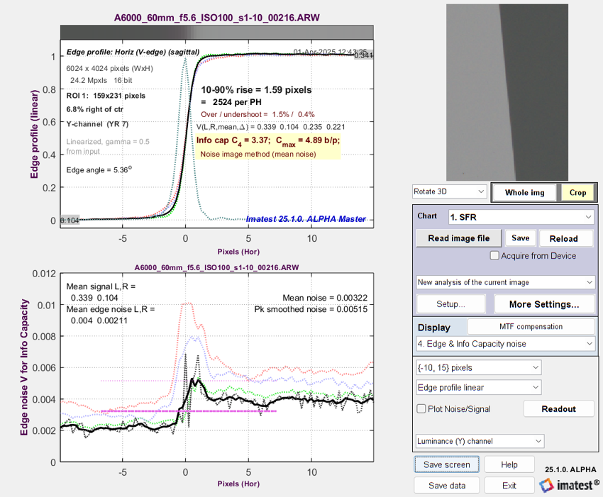 A6000 Edge & Noise plot @ ISO 100 — measured |
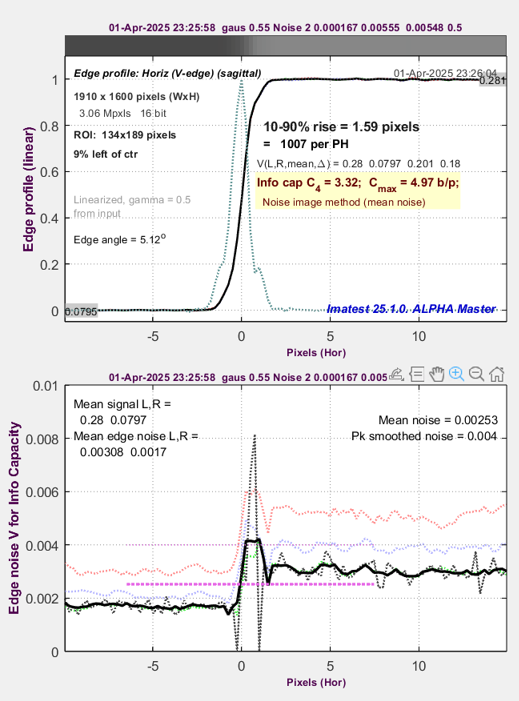 A6000 Edge & Noise @ ISO 100 — simulated |
| Noise is calculated by the MATLAB randn function for each Simatest run. As a result, the noise can look quite different from run-to-run. Here is a different Simatest result for the same settings. Little or no peak is expected when there is no Bilateral filtering. | 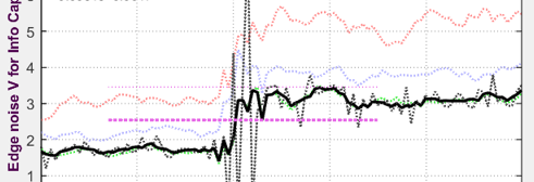 Another run: same settings as above |
|
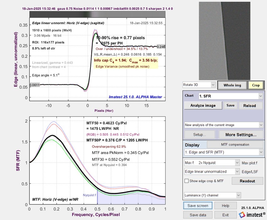
Step 5 – measurement. Repeat Step 3 with just one difference: Increase the Exposure Index to a very high ISO speed (so less light reaches the image sensor and gain is increased). We chose ISO 3200. The ISO 3200 measurement results (MTF curve, information capacities C4 and Cmax, and spatially-dependent noise) are shown on the left, below. |
|
|
Step 6 – simulation. Identical to Step 4, except two lines, shown in dark red, are added to the Simatest ISP blocks: Exposure and 1/EXP, to simulate high ISO speed (low sensor illumination) by multiplying the signal amplitude by 1/32 before applying noise and 32 afterwards.
The measured and simulated Edge and Noise plots are shown on the left and right, below. They are be very close. |
Simatest settings for Rescharts SFR at ISO 3200 (low light) Two lines added. |
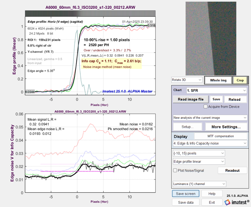 A6000 Edge & Noise plot @ ISO 3200 — measured |
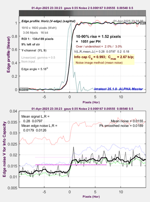 A6000 Edge & Noise @ ISO 3200 — simulated |
The simulation is a great success: measured and modeled performance at ISO 3200 are practically spot-on. They are so close, I had to carefully look at the labels above the plots to see which was which.
Modeling and measuring image sharpness
The next step is to measure and model the image sharpness (SFR or MTF). Since we don’t have the degraded image from a lens design program, we need to estimate the lens blur by trial-and-error using a gaussian or Airy disk filter. Once we have a good model of the raw image, we ae free to try out any adjustments or enhancements.
Since a raw image is required only for finding the noise model, we demosaic (convert) the raw image using LibRaw with the Color 24-bit sRGB preset. The resulting curves are typical for unsharpened images.
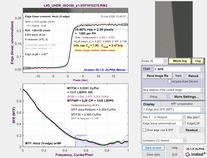 Measured Edge/MTF plot for the Lumix LX5, demosaiced to 24-bit sRGB. Key parameters are 10-90% rise and MTF50.
Simulating image sharpness
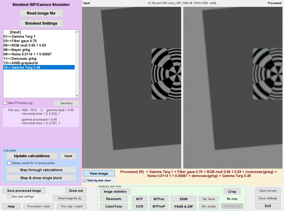
Now we run Simatest, using a demosaiced, minimally processed input image of the 36-patch chart with slanted edges generated by the Imatest Test Charts module.
 Simatest window for matching LX5 simulation with measurement: key setting: Filter gaus 0.75
The following sequence were repeated until we got a good match between the measured Edge/MTF results (above) and the simulated Edge/MTF results.
-
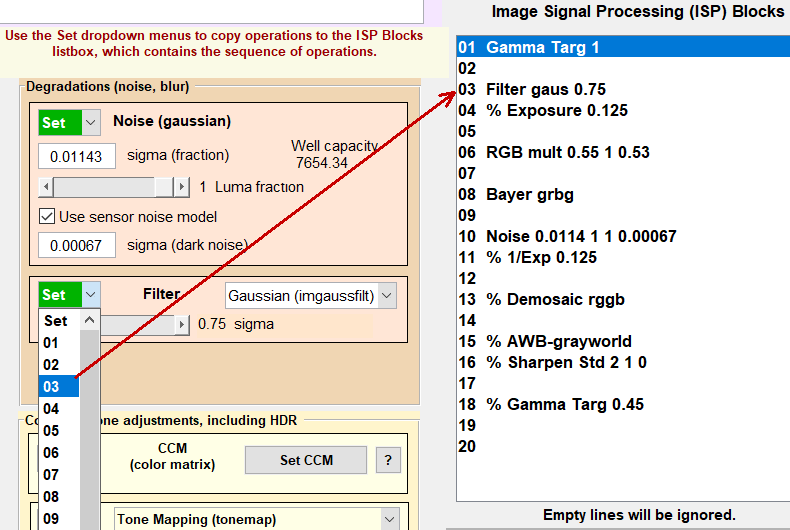
Move the Filter setting to ISP Blocks, line 3.
Click Simatest Settings (upper left of Simatest window). - Filter settings: We tried both Gaussian and Airy disk filters. Gaussian was slightly better, but not perfect. We adjusted the slider several times until we settled on a final value of sigma = 0.75 (pixels).
Recall that Simatest settings require two steps: (1) set the slider (or other adjustment) to the desired value, then (2) press the Set dropdown menu to copy the setting to the selected the line in ISP Blocks, as shown by the red arrow on the right.
- Click OK to return to the main Simatest window.
- Click Update Calculations.
- (optional) You can display the side-by-side view, with the input image on the left and the processed image on the right, shown above. Although this view is occasionally interesting, we typically skip over it.
- Click Rescharts near the bottom of the Simatest window (on the left of the light green area).
- Make sure 1. SFR is chosen for chart, then click on Analyze image.
- Select the region (for the first try) and make a fine adjustment if necessary, or confirm the saved selection (for succeeding tries) by pressing Yes, Express mode.
- If the Edge/MTF plot is selected, the simulated Edge and MTF are displayed. Many other plots are available in both the Rescharts and Color/Tone modules.
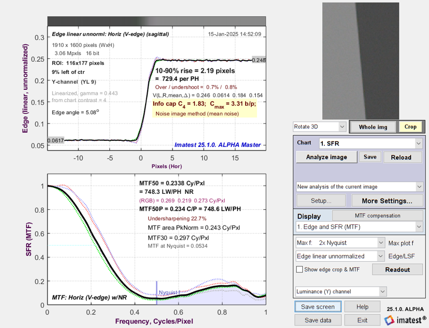 Simulated Edge/MTF plot for the LX5. Results are very close to the measured plot, above.
Key results — 10-90% rise distance, MTF50, Information capacities C4 and Cmax — are all within a few percent.
The match is not perfect. The shape of the MTF is a little off, but it’s good enough for testing ISP.
Simulating the camera JPEG image
Now that we have simulated image sensor noise and the sharpness of a demosaiced, minimally processed image (from the LX5) we can move on to something more challenging: simulating the JPEG image.
Camera JPEGs typically have several additional image processing steps beyond the demosaiced raw image.
- Tonal response curve — can be simple gamma encoding (close to gamma specified for the color space, but sometimes slightly larger to give the image a more snappy appearance).
- Color correction (including White Balance) — Often done by a 3×3 Color Correction Matrix (CCM), but we use simple “gray world” white balance, which is much too simple to handle real-world challenges, in this example.
- Sharpening — standard sharpening (instead of USM) is used in most cameras because it’s faster.
- Noise reduction — typically with a bilateral filter, which keeps edges sharp, but blurs (smooths) the image elsewhere. Bilateral filters are nonuniform and nonlinear. They are nearly universal in consumer camera JPEG images.
- Note that the high quality JPEG image compression in most consumer cameras has little effect on image quality.
Here is the measured JPEG for the LX5, acquired at ISO 100 (Exposure Image).
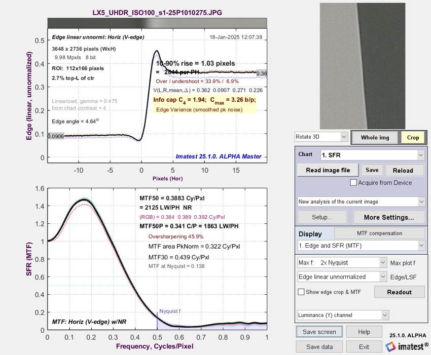 Measured LX5 JPEG Edge/MTF response
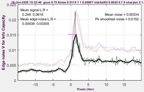
| The second plot is the Edge noise, used to calculate image Information metrics. Edge noise is the lower plot of the Edge & Info Capacity noise display. | 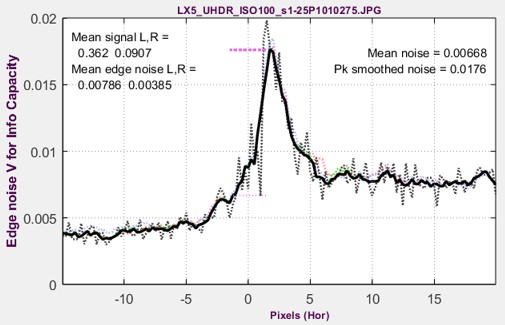 Measured LX5 JPEG Edge noise Measured LX5 JPEG Edge noise |
To simulate this noise, we sharpened the image and applied the MATLAB bilateral filter, which required considerable trial-and-error because it’s not well-documented. Here are the settings.
 Simatest settings for JPEG image
Here is a quick summary of the iterative procedure.
 Simulated LX5 JPEG Edge/MTF response
Results are similar to the measured image, except near fNyq, where MTF is higher.
 Some considerations
- The same input image (from Imatest Test Charts) as the previous simulations was used. The central slanted edge was used to obtain the MTF results.
- Standard sharpening with Radius = 2 and Amount = 1.4 was chosen for a good match to the measured JPEG image. There was some interaction between the sharpening and Bilateral filter settings. To maintain the asymmetry between the larger overshoot and smaller undershoot, sharpening was applied after the encoding gamma (≅0.45) was restored.
- The MATLAB imbilatfilt filter was used. Since Its documentation is not perfectly clear, we had to do a lot of trial-and error to arrive at the settings. We selected Degree of Sharpening = 0.0025, Spatial sigma = 0.7, and Neighborhood area = 5 (must be an odd integer). The noise away from the peak appeared to decrease as Degree of Sharpening was increased.
| These results show how Simatest ISP simulation agrees well (though not perfectly) with measured results. Since we don’t know the properties of the bilateral filter in the LX5, we correctly guessed that it could be approximated by MATLAB imbilatfilt. |
Using the humble Panasonic Lumix LX5 as an example, we have shown how to measure, model and simulate
- image sensor noise, which can be measured from a raw (undemosaiced) image,
- a minimally processed RGB image (converted from raw), and
- a JPEG image (which includes sharpening and bilateral filtering).
The techniques presented here can be used with
- minimally-processed images, converted from raw. These images don’t require the sensor noise or lens blur to be simulated since they’re implicitly included in the image.
- simulated image, especially ideal test chart images. Sensor noise and blur models are required.
- simulated images blurred by a lens design program. The sensor noise model is required.
These cases are illustrated in the block diagram near the beginning of this page.
A great many image processing blocks can be simulated. We have focused on blocks that affect MTF, SFR, noise, information metrics, and color accuracy. The early 2025 release is just a beginning. We expect to add more image processing blocks that customers find useful.